Having a model to predict the performance of a share would be great, wouldn’t it? In this article I will show that such a model indeed exists. From a statistician’s point of view, the rate of stock return follows a particular probability distribution (which is also one of the preconditions of the Black-Scholes model). Assuming that parameters remain stable over a period of time, we can also give probabilities for some rates of stock return. Got curious?
The stock of BASF
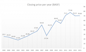
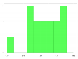
I will illustrate my work using data of BASF’s share. BASF is a huge chemistry company. The left-hand picture below shows the companies share price over the last 16 years. The values correspond to the closing price for each year in Euro (€) . We are interested in the rate of return between the years. The rate of return would equal 1.2 in case the stock increased by 20%, for instance. I prepared a histogram of the stock return rates; it’s shown on the right-hand side.
If you want to produce a forecast regarding a share’s performance, you have to assume a constant probability distribution for the return rates. I chose BASF, because the company is strongly diversified. So, it would take giant fundamental changes to knock out this company. The oil crisis gives a good example on how BASF was less influencable compared to other industries.
Rates of return simulated
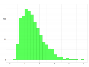
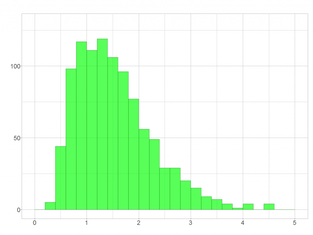
Predicting the rate of stock return for a 5 year interval can easily be accomplished by simulation. Let’s assume that the distribution of returns (shown in the previous section) was the actual probability distrubtion. Drawing a sample of 5 values from this distribution and multiplying them for, say, 1000 times will give an approximately predicition. I performed this kind of resampling and yielded the following distribution.
Recognized the unique shape of the resulting distribution? Statisticians call it a log-normal distribution. Simulation is only a clue, but in the next section you will meet some mathematical background!
Modelling the rate of stock return
As I pointed out, we can model the rate of return over the next years by multiplying the random variables
which represent the rates of return. Then the predicted rate of return
can be stated as follows.
Multiplying random variables is hard. We should try to receive a sum instead. You may come up with the idea of taking the logarithm of both sides of the equation. And that’s fine, because by the loagrithm laws, we can split the logarithm of a product into the sum of the factor’s logarithms 😉
By the central limit theorem, the sum of many (independent!) random variables is distributed normally. Hence, the logarithm of our predicted rate of return – denoted by – may reasonably be normally distributed. Its mean and variance equal the sum of the annual rates’ means and variances. Let’s make
the subject of the above equation, then
However, raising to a normally distributed random power is a perfect definition of the log-normal distribution!
Illustrating theory
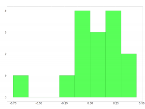
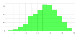
In this section I will give a brief illustration for those who can’t believe that the facts above really hold. 🙂 We first need to take the logarithm of the annual rates of stock return which I presented in the first section (left-hand picture). The sums of each set of 5 values resampled from the logarithmic rates are shown in the right-hand picture. As we are resampling 5 values from a distribution which comprises just 16 values, the result isn’t gorgeous. But you already realize the shape of a normal distribution, don’t you?
Exponentiating results in a log-normal distribution that is similar to the one which we obtained we simulated in the first place:
Deducing a general rule
Now, think about the following: Disregarding the particular distribution of annual return rates we receive a lognormal distribution over a period of 5 years. A year consists of days and therefore must be distributed log-normally. A day, in turn, consists of hours and minutes… See what I try to say? You can assume that rates of return are usually distributed log-normally!
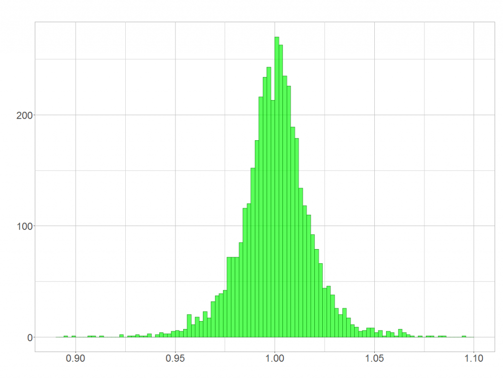
However, when you decrease the time frame’s extent, you’ll probably receive something like this:
This doesn’t look like log-normal, right? Unfortunately, the central limit theorem will make us end up with a ‘looks-like-normal-distribution’, as I have shown in ‘Log-normal distribution mistaken for normal distribution’. Nevertheless, assuming a lognormal distribution is valid in this case.
Further, you may find that the returns around the average are more dense than you would expect from a log-normal distribution (or from a normal distribution of the log-data, respectively). From my point of you, the reasons for this behaviour can be found in the violation of the assumption that returns from different time spans are independent from each other. If nothing happens then… nothing will happen. And so this dense section in the histogram reflects a calm period with not too much action regarding the stock.
On the other hand, selling a huge package of stocks (for whatever reasons) will lower the exchange rate of the stock and will reasonably lead to further sales of this stock by anxious investors. Similar things happen when the exchange rate increases. Other investors beome encouraged to invest and so the price of the stock goes up. You will find evidence for this behaviour in relatively great extreme return rates within the histogram of this stocks’ returns. Therefore, you should not expect a 100% fit of the log-normal distribution. This is also one of the reasons why the Black-Scholes model (for instance) has its limitations.

 (3 votes, average: 4.67 out of 5)





April 1, 2016 at 8:04 am
With log-normal distribution of daily returns what would the annual distribution be?
log-normal(x, 252 * mean(daily_returns), ((252)^0.5) * standard_deviation(daily_returns))
That results in a fat tail of the more positive annual returns.
July 6, 2016 at 8:17 am
To state it in your notation, we would obtain a distribution with
mean: 252 * mean(daily_returns)
variance: 252*(standard_deviation(daily_returns))^2
The shape, however, is not log-normal since (by the central limit theorem) it converges to the shape of the normal distribution. Hence, there won’t be a ‘fat tail of the more positive annual returns’.
October 2, 2016 at 10:16 pm
Why not log-normal? Daily returns should be multiplied, not summed, to get annual return. And a product of log-normal distributions are again log-normal.
October 4, 2016 at 12:08 pm
I am glad that people out there carefully read my articles 🙂 You are perfectly right. I presented my previously reply a long time after producing the article. Obviously there got a mistake in it. The resulting distribution should indeed be log-normal (as stated in the article). If we assume independence of returns, then we can multiply their means.
mean(annual_returns)=mean(daily_returns)^252
You can use the log-transformation and the properties of the normal distribution to find the quantiles of the annual returns. As an example: Since log(daily_returns) is normally distributed, the mean and median are equal. That is, the log-normal distribution of return per year comes with:
median(annual_returns)
=e^(252*mean(log(daily_returns)))
=e^(252*median(log(daily_returns)))
=e^(252*log(median(daily_returns)))
=median(daily_returns)^252
It is interesting that the formula for the annual mean and median resemble each other.