An often forgotten formula for the mean of a random variable 
=\sum_{x=0}^{\infty} \Big(1-F(x)\Big)")
And for the continous case:
=\int_{x=0}^{\infty} \Big(1-F(x)\Big)")
This blog post is going to illustrate how these formulas arise.
Explanation in Discrete Case
Let’s start from the well-known formula for the mean based on the probability mass function (pmf):
Obviously this sum can be extended to include 
=0 \times p(0)=0")
=\sum_{x=1}^{n} x p(x)")
Decomposing the sum we can arrange the involved terms in the form of a triangle:

Graphical representation of the sum of the expected value: Each row gives multiple times the probability mass for a particular x. Therefore each row represents a term of the sum and the highlighted area corresponds to the expected value.
To emphasize what’s going on: Each row consists of multiples of the pmf for some 
Now, we know that the triangle corresponds to the expected value. It doesn’t matter how it is calculated. So, let’s switch from summing rows to summing columns and see what happens!.
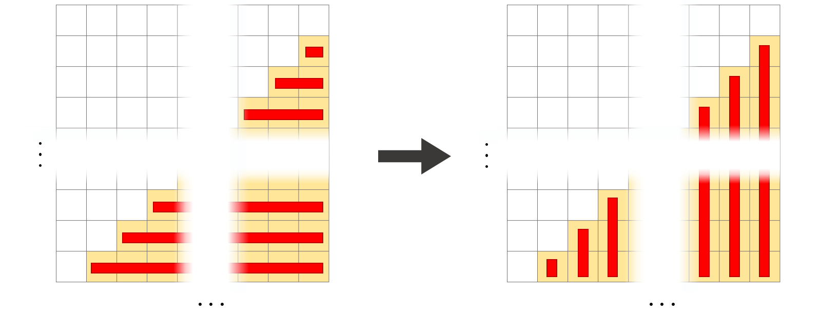
Transition from horizontal to vertical summation: Instead of adding the term row by row, the terms are now added by column. The sum, and thus the expected value, remain the same!
And what does the alternative look like? The point to start at is the fact that the rightmost column adds to 1. The more you move to the right, the more of 1 you lose – in favor of the cumulative distribution function (cdf).
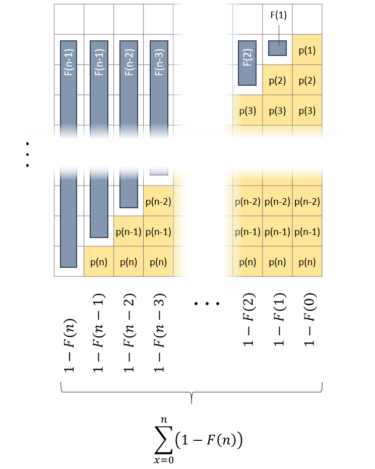
Calculate sum on basis of columns: Still the highlighted area corresponds to the expected value of X. The sum of the rightmost column is equal to 1 as it contains all possible probabilities for X. Moving to the left, each column-sum deaceases as the cumulative distribution function grows. This gives rise to the alternative formula!
On the left-hand end =1")

=0")

Continuous Case
Es finden sich online Beweise, die explizit für die Berechnung des Erwartungswertes kontinuierlicher Zufallsvariablen beschäftigen. Diese haben auch ihre Berechtigung, da sie mithilfe bewiesener Gesetzmäßigkeiten, die Korrektheit folgender Formel belegen:
Für das Verständnis ist es aber sicher sinnvoller, sich vorzustellen, dass man die Formel des vorangegangenen Abschnitts auf unendlich viele unendlich kleine ")


Leave a Reply