In applied statistics you often have to combine data from different samples or distributions. One of the most frequently used operation here is to add means and expected values. For instance, you could sample people’s leg length, body and head height. The result when adding these means? It is the average body height, I hope!
Relationship between expected value and mean
My reasoning, why adding means works, will be based on expected values. The expected value of a random variable is defined as
![\displaystyle \mathrm{E}[X]=\sum \limits_{x} x \times p_{x}(x)](http://s0.wp.com/latex.php?latex=%5Cdisplaystyle+%5Cmathrm%7BE%7D%5BX%5D%3D%5Csum+%5Climits_%7Bx%7D+x+%5Ctimes+p_%7Bx%7D%28x%29&bg=ffffff&fg=000000&s=0 "\displaystyle \mathrm{E}[X]=\sum \limits_{x} x \times p_{x}(x)")
where ")

![\displaystyle \overline{x}=\frac{1}{n} \sum\limits_{x} x=\sum\limits_{x} \frac{x}{n} \approx \mathrm{E}[X]](http://s0.wp.com/latex.php?latex=%5Cdisplaystyle+%5Coverline%7Bx%7D%3D%5Cfrac%7B1%7D%7Bn%7D+%5Csum%5Climits_%7Bx%7D+x%3D%5Csum%5Climits_%7Bx%7D+%5Cfrac%7Bx%7D%7Bn%7D+%5Capprox+%5Cmathrm%7BE%7D%5BX%5D&bg=ffffff&fg=000000&s=0 "\displaystyle \overline{x}=\frac{1}{n} \sum\limits_{x} x=\sum\limits_{x} \frac{x}{n} \approx \mathrm{E}[X]")
Mean or expected value; the subsequent explanation is valid either way.
Adding two random variables
Now let’s assume we wanted to add two random variables – say 

")


=P\big(X=x, Y=y\big)")
With two variables we now have to process all possible combinations of 
![\displaystyle \mathrm{E}\big[X+Y\big]=\sum\limits_{x} \sum\limits_{y} (x+y) \times p_{x,y}(x,y)=\sum\limits_{x} \sum\limits_{y} \big(x \times p_{x,y}(x,y)+y \times p_{x,y}(x,y)\big)](http://s0.wp.com/latex.php?latex=%5Cdisplaystyle+%5Cmathrm%7BE%7D%5Cbig%5BX%2BY%5Cbig%5D%3D%5Csum%5Climits_%7Bx%7D+%5Csum%5Climits_%7By%7D+%28x%2By%29+%5Ctimes+p_%7Bx%2Cy%7D%28x%2Cy%29%3D%5Csum%5Climits_%7Bx%7D+%5Csum%5Climits_%7By%7D+%5Cbig%28x+%5Ctimes+p_%7Bx%2Cy%7D%28x%2Cy%29%2By+%5Ctimes+p_%7Bx%2Cy%7D%28x%2Cy%29%5Cbig%29+&bg=ffffff&fg=000000&s=0 "\displaystyle \mathrm{E}\big[X+Y\big]=\sum\limits_{x} \sum\limits_{y} (x+y) \times p_{x,y}(x,y)=\sum\limits_{x} \sum\limits_{y} \big(x \times p_{x,y}(x,y)+y \times p_{x,y}(x,y)\big)")
We can split the right-hand side into two separat sums. As it doesn’t matter whether you sum the values for
![\displaystyle \mathrm{E}\big[X+Y\big]=\sum\limits_{x} \sum\limits_{y} x\times p_{x,y}(x,y)+ \sum\limits_{x} \sum\limits_{y} y\times p_{x,y}(x,y)](http://s0.wp.com/latex.php?latex=%5Cdisplaystyle+%5Cmathrm%7BE%7D%5Cbig%5BX%2BY%5Cbig%5D%3D%5Csum%5Climits_%7Bx%7D+%5Csum%5Climits_%7By%7D+x%5Ctimes+p_%7Bx%2Cy%7D%28x%2Cy%29%2B+%5Csum%5Climits_%7Bx%7D+%5Csum%5Climits_%7By%7D+y%5Ctimes+p_%7Bx%2Cy%7D%28x%2Cy%29&bg=ffffff&fg=000000&s=0 "\displaystyle \mathrm{E}\big[X+Y\big]=\sum\limits_{x} \sum\limits_{y} x\times p_{x,y}(x,y)+ \sum\limits_{x} \sum\limits_{y} y\times p_{x,y}(x,y)")
![\displaystyle \mathrm{E}\big[X+Y\big]=\sum\limits_{x} \sum\limits_{y} x\times p_{x,y}(x,y)+ \sum\limits_{y} \sum\limits_{x} y\times p_{x,y}(x,y)](http://s0.wp.com/latex.php?latex=%5Cdisplaystyle+%5Cmathrm%7BE%7D%5Cbig%5BX%2BY%5Cbig%5D%3D%5Csum%5Climits_%7Bx%7D+%5Csum%5Climits_%7By%7D+x%5Ctimes+p_%7Bx%2Cy%7D%28x%2Cy%29%2B+%5Csum%5Climits_%7By%7D+%5Csum%5Climits_%7Bx%7D+y%5Ctimes+p_%7Bx%2Cy%7D%28x%2Cy%29&bg=ffffff&fg=000000&s=0 "\displaystyle \mathrm{E}\big[X+Y\big]=\sum\limits_{x} \sum\limits_{y} x\times p_{x,y}(x,y)+ \sum\limits_{y} \sum\limits_{x} y\times p_{x,y}(x,y)")
This is where it gets tricky. On the one hand, we can drag
![\displaystyle \mathrm{E}\big[X+Y\big]=\sum\limits_{x} x \times \sum\limits_{y} p(x,y)+ \sum\limits_{x} y\times \sum\limits_{y} p(x,y)](http://s0.wp.com/latex.php?latex=%5Cdisplaystyle+%5Cmathrm%7BE%7D%5Cbig%5BX%2BY%5Cbig%5D%3D%5Csum%5Climits_%7Bx%7D+x+%5Ctimes+%5Csum%5Climits_%7By%7D+p%28x%2Cy%29%2B+%5Csum%5Climits_%7Bx%7D+y%5Ctimes+%5Csum%5Climits_%7By%7D+p%28x%2Cy%29+&bg=ffffff&fg=000000&s=0 "\displaystyle \mathrm{E}\big[X+Y\big]=\sum\limits_{x} x \times \sum\limits_{y} p(x,y)+ \sum\limits_{x} y\times \sum\limits_{y} p(x,y)")
Further we can simplify the probabilities. See, adding ")
")
![\displaystyle \mathrm{E}\big[X+Y\big]=\sum\limits_{x} x \times p_{x}(x)+ \sum\limits_{y} y\times p_{y}(y)](http://s0.wp.com/latex.php?latex=%5Cdisplaystyle+%5Cmathrm%7BE%7D%5Cbig%5BX%2BY%5Cbig%5D%3D%5Csum%5Climits_%7Bx%7D+x+%5Ctimes+p_%7Bx%7D%28x%29%2B+%5Csum%5Climits_%7By%7D+y%5Ctimes+p_%7By%7D%28y%29+&bg=ffffff&fg=000000&s=0 "\displaystyle \mathrm{E}\big[X+Y\big]=\sum\limits_{x} x \times p_{x}(x)+ \sum\limits_{y} y\times p_{y}(y)")
But what do we have here? Each of the right-hand side’s terms is equal to the definition of an expected value!
![\mathrm{E}\big[X+Y\big]=\mathrm{E}\big[X\big] + \mathrm{E}\big[Y\big]](http://s0.wp.com/latex.php?latex=%5Cmathrm%7BE%7D%5Cbig%5BX%2BY%5Cbig%5D%3D%5Cmathrm%7BE%7D%5Cbig%5BX%5Cbig%5D+%2B+%5Cmathrm%7BE%7D%5Cbig%5BY%5Cbig%5D&bg=ffffff&fg=000000&s=0 "\mathrm{E}\big[X+Y\big]=\mathrm{E}\big[X\big] + \mathrm{E}\big[Y\big]")
Some comments
The last equation has shown that we can, indeed, add expected values. Have you noticed that we didn’t make any assumptions regarding the independence of the random variables? Hence, the rule holds even if your random variables are correlated! And remember the introductory example? We used a continous measure there. Just replace all sum signs by integral signs and you’ll see that the rule works with continous random variables too.
Always keep in mind that you can apply the addition to means as well. So, the mean 


 (4 votes, average: 4.75 out of 5)


Leave a Reply